Neural networks: Functions that learn
In 1989, researchers at Bell Labs built a system to read handwritten ZIP codes off envelopes. The dataset they eventually assembled — 70,000 grayscale images of handwritten digits, called MNIST — became the “hello world” of machine learning, and it’s where we’ll start too.
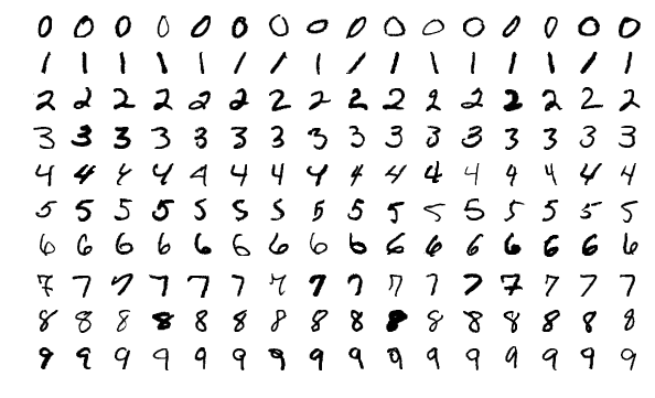 Samples from MNIST. Image by Josef Steppan , CC BY-SA 4.0.
Programming with data
Programming a computer to read these scribbles is brutally hard with classical logic. There are no hard-and-fast rules for what makes a 5 a 5 — every rule you write has a thousand exceptions — and the early vision systems built on hand-written rules fell on their faces. The same wall appears wherever the input is fuzzy: parsing an English sentence, recognizing a face in a photo. This is why these problems stayed unsolved for decades while computers conquered chess. But problems like these have a saving grace: the rules are hard to write, but examples are cheap — and the discipline for extracting patterns from examples is statistics.
That’s the thread this chapter pulls on, in three steps:
- We treat digit-reading as a statistics problem. The simplest statistical tool is a regression — give every pixel a weight, add up the evidence — and this alone reads 92% of digits correctly.
- But a regression is linear: it can weigh each pixel, but it can’t see combinations of strokes. Stacking regressions with small decisions between them — a neural network — lets us learn arbitrary functions, not just linear ones.
- “Learning” means searching for good values of the weights. Gradient descent does the searching — measure how wrong the current weights are and follow the slope downhill — and the chain rule (backpropagation) is what makes computing that slope cheap, even for millions of weights.
Seen this way, machine learning is a different way to program a computer: instead of writing the function yourself, you write its signature (an architecture with millions of tunable parameters), define what “good output” looks like (a loss function), and let an optimization algorithm fill in the implementation.
One piece of vocabulary before we build: a model’s life has two distinct phases. Training is when the optimization algorithm is searching for good weights — the model is being written. Inference is everything after: the weights are frozen, and the model is simply being used, like any other function. This chapter is almost entirely about training; by the end of the book, inference will have earned three chapters of its own.
The model: from a matrix to an MLP
Back to MNIST — an MNIST image is 28×28 pixels. Flatten it and you get a vector of 784 numbers between 0 (white) and 1 (black). We want a function that maps that vector to an answer: which digit is this?
Notice that the problem itself isn’t deterministic. A sloppily written 5 shades into a 2; even humans disagree about the worst examples. So a function that returns the answer is the wrong shape — what we want is a function that weighs the evidence and returns a score for each of the 10 candidates, which we can treat as (and will shortly convert into) probabilities. Again, we’re doing statistics, not logic.
The simplest mechanism in all of statistics for turning many weighted pieces of evidence into a score is a regression — a linear function of the input:
where is a 10×784 matrix of weights and is a vector of 10 biases. Each row of is effectively a template: the dot product between the input and that row measures “how much does this image look like this row’s digit.” This alone — a linear classifier — gets about 92% accuracy on MNIST, which tells you something important: a matrix multiply is already a primitive form of pattern matching.
Why does a linear model top out at 92%? Because of what linearity means: each pixel gets one fixed weight, votes independently, and the votes are simply added up. A linear model cannot express “this pixel is evidence for an 8 — but only if this other region is dark too.” The pixels of a 5 and a 2 overlap heavily; what distinguishes them is the combination of strokes, and combinations are exactly what a weighted sum can’t see. In programming terms: a linear function is a program with no if statements — one pass of weighted arithmetic, no decisions that depend on the input.
You might try to fix this by stacking two linear layers. But composing linear functions just gives you another linear function ( — the composition collapses into one matrix). However many layers you stack, you’ve written a longer program with still no if statements.
The fix is to insert a nonlinearity between the layers, and the field has settled on the almost comically simple ReLU : . Look at what it does: below zero the unit outputs nothing; above zero it passes its signal through. That’s a branch — the smallest possible if. With a nonlinearity between them, the layers stop collapsing: the first layer can compute features, the ReLU can decide which ones are present, and the second layer can weigh combinations of those decisions.
Stack linear layers with nonlinearities between them and you have a multi-layer perceptron (MLP):
With one hidden layer of 512 units, this gets ~98% on MNIST. Intuitively, the first layer learns to detect features (strokes, loops, corners), and the second layer learns to combine features into digits.
But stacking the layers broke something important. A lone regression can be solved: for a linear model, calculus hands you the best-fit weights directly — set the derivative of the error to zero and solve the equations (this is least squares, the same machinery that fits a trend line in a spreadsheet). The moment a nonlinearity sits between two matrices, that machinery dies. For a linear model the error surface is a smooth bowl — “set the derivative to zero” is a system of linear equations with one solution. Add the ReLUs and the surface shatters into an exponential number of pieces, and “set the derivative to zero” becomes a system of nonlinear equations nobody can solve in general. This isn’t just empirical pessimism: Blum and Rivest proved that optimally training even a three-neuron network is NP-complete, so a general-purpose recipe for the best and would, among other things, resolve P vs. NP. The best anyone knows how to do is start with random weights and improve them iteratively — which is exactly what the rest of this chapter is about.
The learning: gradient descent
So here’s where we are: an MLP with ~400,000 weights, every one of them initialized to a random number. Feed it our 7 and it reports something like 10% on every digit — of course it does; it’s random. How do we get 400,000 random numbers to take on useful values?
Since we can’t solve for them, we iterate: nudge the weights, check whether the model got better, keep the nudges that help, repeat a few hundred thousand times. For now, assume that “did the model get better?” is a single number we can compute — a score, called the loss , that measures how wrong the model is on the training data, where lower is better. (Constructing it carefully is the next section’s job; here we only need that it exists and is smooth.)
Here’s the situation for any single weight. Somewhere out there is its optimal value — the setting that makes the model least wrong. We don’t know how to find it; that’s the closed-form door that slammed shut a section ago. What we do know how to compute, for whatever value we currently have, is how bad it is (the loss) — and, because the loss is smooth, which direction makes it worse (the derivative). That suggests a humble strategy: repeatedly move in whichever direction makes things less bad, and stop when no direction helps. You may never learn where the best value was, but you’ll settle somewhere least bad.
Scaled up to all 400,000 weights at once, this is gradient descent: compute the gradient of the loss — the direction that increases it fastest — and take a small step the other way.
This update runs for every weight simultaneously. Each weight’s partial derivative, collected into one big vector, is the gradient — papers write the whole update as , and now you can read that too.
Why a small step — and why must the steps shrink as we close in? Imagine taking the same confident stride every time: nearing the valley floor, you’d overshoot it, land on the opposite slope, turn around, and overshoot again — orbiting the minimum forever without ever landing on it. Gradient descent has an elegant built-in fix: the step is times the slope, and the slope fades to zero at the minimum, so the steps shrink automatically as you arrive — exactly what the animation above shows. Here’s the fixed-stride version for comparison:
The multiplier is the learning rate, and it is the single most finicky number in all of deep learning. Too small is merely slow — thousands of timid steps down a hill you could have descended in ten. Too large is fatal, and it’s worth seeing exactly why, because it seems to contradict the self-shrinking steps we just celebrated. That guarantee had a hidden assumption: that each step lands you closer to the minimum, where the slope is gentler and the next step therefore smaller. Overshoot far enough, though, and you land on the far slope at a point steeper than the one you left. Now “step proportional to slope” works against you: a steeper landing means a bigger next step, which means a steeper landing still. The same feedback loop that damped the walk now amplifies it, and the parameters ricochet outward until the numbers overflow. On our parabola you can make this exact: each step multiplies your distance from the minimum by a fixed factor set by — below the threshold that factor is less than one and the walk converges; above it, every step pushes you further away than you started.
Two practical modifications matter:
- Stochastic gradient descent (SGD — the name you’ll see in every framework and paper): you could compute the exact gradient over all 60,000 images before each step — but consider what that buys you. The gradient from a random sample of images is an unbiased estimate of the full gradient, and its accuracy improves only with the square root of the sample size, while its cost grows linearly. Worse, extra precision is mostly thrown away: you only take one small step in that direction, and after the step the landscape has changed and the direction must be recomputed anyway. So instead, estimate the gradient on a random batch (say, 128 images) per step: for the price of one perfect step you take ~500 noisy ones, and 500 stumbles downhill travel much farther than one flawless stride. (The noise even turns out to help — it jiggles the trajectory out of flat regions and bad ruts.)
- Epochs: one full pass through the training data is an epoch. Small datasets get looped over many times. (Foreshadowing: LLMs, trained on trillions of tokens, typically see their data roughly once — more on that in Chapter 7.)
The loss: measuring wrongness
Now let’s construct the number we’ve been assuming. Gradient descent quietly imposed two requirements on it: the loss must be differentiable (we take its gradient), and it should change continuously as the model improves (a compass that only moves in rare jumps gives the search no direction). Defining it well matters as much as the architecture does — it is, literally, the spec the model will be optimized against.
Those requirements immediately disqualify the obvious candidate: accuracy, percent correct. Nudge one weight slightly and usually no prediction flips, so accuracy doesn’t move at all — flat almost everywhere, gradient zero, no signal. What we want instead is a number that rewards moving from “99% sure it’s a 3” to “60% sure it’s a 3” on an image of a 5, even though both are, discretely, the same mistake. That means grading the model’s confidence, not just its verdict — and for that, its outputs need to be probabilities.
The 10 output scores (called logits) are unbounded real numbers. To interpret them as a probability distribution, we pass them through softmax:
Softmax exponentiates each score (making everything positive, and amplifying differences) and normalizes so they sum to 1. Here it is applied to the scores our linear classifier produced for the 7:
The target it’s graded against is the label written as a one-hot vector — all zeros except a 1 on the correct digit: a probability distribution with all of its mass on the truth. The grading rule is cross-entropy loss: the negative log of the probability the model assigned to the correct answer.
The log of a probability has a name you’ll meet in every LLM API: a logprob. Probabilities live in [0, 1], so logprobs live in [−∞, 0] — zero when the model is certain, increasingly negative as it’s surprised — and cross-entropy is just the correct answer’s logprob, negated. If the model puts probability 1 on the right answer, the loss is 0. If it puts probability 0.01 on it, the loss is ~4.6.
Why the log, rather than something simpler like penalizing ?
One statistical reason and one practical one. Statistically, the natural goal is to maximize the probability of getting the whole training set right — and since that’s a product of 60,000 per-example probabilities, it’s hopeless to work with directly (it would underflow any floating-point format, and calculus hates products). Taking the log turns the product into a sum of per-example terms — exactly our loss — without changing what’s being maximized.
Practically, the log changes how wrongness is punished: a linear penalty barely distinguishes “wrong at 1%” from “wrong at 0.001%”, so the gradient fades just when correction is most needed. Under the log, every additional order of magnitude of overconfident wrongness costs the same again — the loss stays fierce precisely where the model is most confidently wrong.
(There’s a third, deeper reading — the logprob is the number of bits needed to encode the right answer under the model’s beliefs — that pays off next chapter, when training a language model turns out to be compression.)
Averaged over the dataset, this single number summarizes how wrong the model is — smooth, differentiable, and falling steadily as confidence shifts toward the right answers. “Learn to read digits” has become “minimize this function.”
Backpropagation: the chain rule, industrialized
How do you compute a gradient with respect to a million parameters? First, a term: running the network front-to-back — pixels in, through the layers, predictions out — is called a forward pass; it’s what the model does every time it makes a prediction (during training, we then score those predictions against the label to get the loss).
Backpropagation computes all of the gradients in about the cost of two forward passes. The engine is the chain rule from calculus. As a reminder: when functions are composed, their rates of change multiply. Take the simplest case from our own network — the loss depends on the prediction , and the prediction depends on some weight . Then:
Nudge the weight: its effect on the prediction is scaled by , and that effect on the loss is scaled again by — two links in a chain, two factors in a product. A deep network is just a longer chain.
Backprop computes every weight’s derivative — exactly, not by estimate — in one sweep:
- One forward pass, keeping every intermediate value (, , , ) in memory instead of discarding them.
- One backward sweep. Start at the loss and walk the network back to front. At each value, compute “how much does the loss change if this changes” — which is cheap, because it’s just the answer already computed for the value after it, times one local derivative. And the local derivatives are known analytically: every operation in the network is simple (multiply, add, relu, softmax), and calculus gives each one’s derivative as a formula — evaluated instantly using the values remembered from the forward pass. No anywhere.
- Collect the gradients along the way. Every time the sweep passes a weight, that weight’s exact falls out as a byproduct. By the time it reaches the input, you hold the derivative for all 400,000 weights — from one backward walk that costs about as much as the forward one.
Here is the whole thing running on a tiny two-layer network, with real numbers — four forward calculations, then four backward, one per step:
| value | ∂L/∂· | |
|---|---|---|
| w₁₁ | 0.5 | · |
| w₂₁ | 1 | · |
| w₁₂ | 1 | · |
| w₂₂ | −1 | · |
| v₁ | 1 | · |
| v₂ | 2 | · |
| h₁ | 2 | · |
| h₂ | · | · |
| ŷ | · | · |
| L | · | · |
Watch what the backward pass reuses: is computed once and feeds every gradient below it; each is computed once and feeds every weight into that unit. That reuse is the dynamic programming — and it’s how a million gradients cost about the same as two forward passes instead of a million.
Then gradient descent acts on all of them simultaneously: every weight takes its own step, scaled by its own partial derivative — , applied to all 400,000 at once. One forward pass, one backward pass, one synchronized update: that is a training step, and a training run is millions of them.
In practice you never write this by hand. Frameworks like PyTorch record the computational graph as your code runs and derive the backward pass automatically (this is “autograd”). Here is the entire training loop, for real:
model = nn.Sequential(
    nn.Linear(784, 512),
    nn.ReLU(),
    nn.Linear(512, 10),
)
opt = torch.optim.SGD(model.parameters(), lr=0.1)

for images, labels in dataloader:          # batches of 128
    logits = model(images.view(-1, 784))   # forward pass
    loss = F.cross_entropy(logits, labels) # softmax + neg-log-likelihood
    opt.zero_grad()
    loss.backward()                        # backprop: fills in .grad
    opt.step()                             # gradient descent step
Every model in this book — up to and including the frontier ones — is trained by a scaled-up version of these ten lines.
Better optimizers: momentum and Adam
Vanilla SGD — gradient descent on random batches, exactly as we’ve described it — works, but the loss landscape of a real network is a mess of ravines and plateaus, and two refinements are so universal you should know them by name.
Momentum keeps a running average of recent gradients and steps in that direction — like a ball rolling downhill, it smooths over noise and powers through small bumps.
Adam additionally tracks a running average of the gradient’s magnitude for each individual parameter, and scales each parameter’s step size accordingly: parameters with consistently large gradients get smaller steps, and vice versa. It’s a per-parameter adaptive learning rate. The variant actually used everywhere is AdamW , which fixes how weight decay (a regularization term) interacts with the adaptivity.
What’s weight decay, and what exactly did AdamW fix?
Weight decay is a gentle pressure that shrinks every weight slightly toward zero on each step — multiply each one by, say, 0.9999 before the update. Why want that? Large weights make a network twitchy: small changes in the input swing the output hard, which is the signature of a model contorting itself to memorize. Keeping weights small unless the data genuinely earns them is a classic guard against overfitting.
The subtle bug AdamW fixed: the traditional implementation of weight decay adds the shrinking pressure into the gradient. Under plain SGD those two formulations are mathematically identical. Under Adam they are not — Adam divides every gradient by its running magnitude, and the decay term gets divided along with it. The result: weights with large, active gradients barely decay, while quiet weights decay hard. The regularization strength you set silently varies from parameter to parameter.
AdamW decouples the two (the paper is literally titled “Decoupled Weight Decay Regularization”): the gradient goes through Adam’s adaptive machinery, and the decay is applied to the weights directly, outside it. Same ingredients, consistent regularization — and the default optimizer of every LLM config since.
When you read an LLM paper and see “AdamW, β₁ = 0.9, β₂ = 0.95,” those betas are just the decay rates of the two running averages. One consequence worth filing away for the infrastructure chapters: Adam stores two extra numbers per parameter, so the optimizer’s state is twice the size of the model itself.
Putting it together: learning XOR
Every piece is now on the table, so let’s watch a complete training run — on a problem a linear model provably cannot solve. XOR (“exactly one of the two inputs is on”) is the famous one: no single weighted sum separates its positives from its negatives, a fact that stalled neural network research for a decade. Two hidden neurons and a ReLU handle it.
The network below is as small as they come — two inputs, two hidden units, one output squashed through a sigmoid (softmax’s two-option sibling, turning the score into a probability between 0 and 1). It trains on all four cases of XOR at once, by plain gradient descent:
| x₁ | x₂ | target | ŷ |
|---|---|---|---|
| 0 | 0 | 0 | 0.50 |
| 0 | 1 | 1 | 0.50 |
| 1 | 0 | 1 | 0.46 |
| 1 | 1 | 0 | 0.34 |
| mean loss | 0.228 | ||
| param | value | ∂L/∂· |
|---|---|---|
| w₁₁ | 0.70 | · |
| w₂₁ | 0.80 | · |
| b₁ | 0.00 | · |
| w₁₂ | 0.90 | · |
| w₂₂ | 0.80 | · |
| b₂ | -0.40 | · |
| v₁ | 0.60 | · |
| v₂ | -1.20 | · |
| c | 0.00 | · |
Early on, the gradients are large and the weights move fast; by the end, the predictions hug their targets and the gradients fade toward zero — the walk settling into the bottom of the bowl, visible as a table of numbers instead of a curve.
What training actually looks like
On paper, training is “run the loop until the loss is low.” In practice, training is staring at the loss curve — and knowing what to check, in what order, when it isn’t doing what you want. For our MNIST net, the ritual looks like this:
First number: the loss at initialization. Before any training, a 10-class model with random weights should assign roughly 10% to everything, so its cross-entropy should be almost exactly . Check it. If it’s 7, your initialization is broken; if it’s 0.3, you have a bug (probably your data is leaking the answer). This one free sanity check catches a remarkable fraction of setup errors before you’ve spent a single GPU-minute.
First milestone: overfit one batch. Take 32 images and train on just those until the loss is ~0. Here’s why that’s possible: with 400,000 adjustable weights and only 32 examples, the network has vastly more capacity than the task needs, so gradient descent can simply memorize the right answer for each one — brute-forcing the loss to zero without learning anything general. Normally memorization is the failure mode you fight (the next section is about exactly that); here it’s a diagnostic. A network that can’t memorize 32 examples has a plumbing problem — wrong shapes, a broken loss, gradients not flowing. Skipping this step is the classic way to spend a day debugging the wrong layer of the stack.
Then: watch the shape. With the plumbing verified, start real training and read the curve. There are only three shapes, and the learning rate usually picks between them:
When the curve diverges, lower the learning rate; when it crawls, raise it. The standard move is a sweep over powers of ten — nobody, at any level of seniority, guesses it correctly on the first try. For our MNIST MLP, a healthy run takes the loss from 2.3 to under 0.1 within a couple of epochs, and accuracy to ~98%.
What matters, in order. For a fixed dataset, the learning rate dwarfs everything else; after that, training longer and making the model bigger; after that, the architecture tweaks people love to argue about. And looming over all of it: more and better data beats all of the above — a hierarchy so reliable it becomes the thesis of Chapter 4. Karpathy’s A Recipe for Training Neural Networks is the canonical write-up of this discipline, and it transfers almost unchanged from MNIST to frontier models.
There’s one curve we haven’t mentioned yet, though — and it’s the one that actually matters.
Generalization: the point of all this
One last concept, because it’s the difference between machine learning and curve fitting. A model with enough parameters can memorize its training set — and score 100% on it while being useless on new data. This is overfitting, and it’s why we always hold out a test set the model never trains on, and report accuracy there. In practice you watch two loss curves during training — one on training data, one on held-out data — and the number you actually care about is the second. When the training curve keeps falling but the held-out curve turns back upward, the model has stopped learning and started memorizing.
The entire game is generalization: we don’t want a model that knows these 60,000 digits, we want one that has learned what digits are. Keep this tension in mind — it returns with a vengeance when we discuss benchmark contamination in Chapter 9.
Further reading
- Neural Networks: Zero to Hero — Karpathy’s video series building all of this (including autograd) from scratch in Python. The single best resource for making this chapter concrete.
- Yes you should understand backprop — why backprop is a leaky abstraction worth understanding even though frameworks do it for you.
- 3Blue1Brown’s neural network series — the best visual intuition for gradient descent and backprop ever produced.
- Adam and AdamW — the optimizer papers; skimmable, and useful for decoding the hyperparameter tables in every LLM technical report.